PDFNORM

Purpose:

Returns the probability density function for a normal distribution.

Syntax:

PDFNORM(z, mean, std)

z	-	A real or series. The z value.
mean	-	Optional. A real, the mean of the distribution. Defaults to 0.0.
std	-	Optional. A real, the standard deviation of the distribution, where std > 0. Defaults to 1.0.

Returns:

A real or series, the value of the normal distribution function for the given mean and standard deviation.

Example:

pdfnorm(0)

returns 1, the value of the normal distribution with a mean of 0.0 and a standard deviation of 1.0.

Example:

pdfnorm(-8..0.01..8)

displays the normal distribution with a mean of 0.0 and a standard deviation

of 1.0 over the range -8 to 8.

Example:

pdfnorm(-8..0.01..8, 0, 2.0)

Same as above except the standard deviation of the distribution is set to 2.0.

Example:

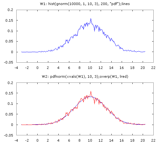
W1: hist(gnorm(10000, 1, 10, 3), 200, "pdf");lines

W2: pdfnorm(xvals(W1), 10, 3);overp(W1, lred)

Compares the calculated normal distribution of random values with mean 10 and standard deviation 3 in W1 with the analytic distribution in W2. The overplotted histogram is normalized to provide an visual accurate comparison.

Remarks:

The result is NaN where std ≤ 0.

The probability density function, f(x), for normally distributed random values is:

where μ is the mean, σ is the standard deviation and σ² is the variance. The cumulative distribution function, Φ(x), is:

where erf(x) is the error function implemented by ERF.

Approximately 68% of the values from a normal distribution are within one standard deviation away from the mean. Approximately 95% of the values lie within two standard deviations and approximately 99.7% are within three standard deviations. This is known as the 3-sigma rule.

See PROBN to calculate the normal cumulative distribution function.

See GNORMAL to generate a series of normally distributed random values.

PDFNORM

Purpose:

Syntax:

Returns:

Example:

Example:

Example:

Example:

Remarks:

See Also: