DADiSP Online Help
Click here to see this page in full context

DADiSP Worksheet Functions > Function Categories > Statistics and Calculus > HISTOGRAM
Creates a histogram of the input series.
HISTOGRAM(series, nbins, width, offset, "normalization")
|
series |
- |
Any series, table, or expression evaluating to a series or table. |
||||||||||||
|
nbins |
- |
An integer, the number of bins. |
||||||||||||
|
width |
- |
Optional. A real, the width of each bin if |
||||||||||||
|
offset |
- |
Optional. A real, the starting bin edge if |
||||||||||||
|
"normalization" |
- |
Optional. A string, the normalization method:
|
HISTOGRAM(series, edges, "normalization")
|
series |
- |
Any series, table, or expression evaluating to a series or table. |
||||||||||||
|
edges |
- |
A series, a list of bin edges. |
||||||||||||
|
"normalization" |
- |
Optional. A string, the normalization method:
|
A series or table displayed as a bar chart.
histogram({3, 5, 1, 7, 4, 5, 7, 3, 1, 9}, 10)
returns a series {2, 0, 2, 1, 2, 0, 0, 2, 0, 1} displayed in bar chart format.
histogram({3, 5, 1, 7, 4, 5, 7, 3, 1, 9}, -1, 0.8, 1.0)
same result as above except the bin width is explicitly specified as 0.8 and the starting bin is 1.0 .
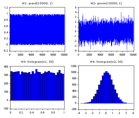
W1: grand(10000, 1)
W2: gnorm(10000, 1)
W3: histogram(w1, 30)
W4: histogram(w2, 30)

W3 and W4 graphically demonstrate the distributions of uniform random noise and normally distributed random noise.
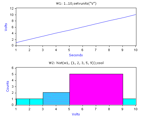
W1: 1..10;setvunits("V")
W2: hist(w1, {1, 2, 3, 5, 9});cool

Creates a shaded histogram with the following bin attributes:
|
Bin Edges |
Bin Counts |
|
1 <= bin1 < 2 |
1 |
|
2 <= bin2 < 3 |
1 |
|
3 <= bin3 < 5 |
2 |
|
5 <= bin4 < 9 |
5 |
|
9 <= bin5 <= 10 |
1 |
W1: gnorm(10000, 1, 2, 5)
W2: pdfnorm(-25..0.01..25, 2, 5)
W3: hist(w1, 50, "pdf");overp(w2, lred)
W1 contains 10000 samples of normally distributed values with a mean of 2 and a standard deviation of 5.
W2 computes the probability distribution of a normal distribution with a mean of 2 and a standard deviation of 5.
W3 creates a 50 sample histogram normalized based on the PDF. The analytic distribution is overplotted for comparison.
W1: gnorm(10000, 1, 2, 5)
W2: gnorm(1000, 1, 10, 5)
W3: hist(w1, 30, "prob")
W4: hist(w2, 30, "prob");overp(w3, lred)
W1 contains 10000 samples of normally distributed values with a mean of 2 and a standard deviation of 5.
W2 contains 1000 samples of normally distributed values with a mean of 10 and a standard deviation of 5.
W3 creates a 30 sample histogram of W1 normalized such that the sum of the histogram is 1.
W4 creates a 30 sample histogram of W2 normalized such that the sum of the histogram is 1. The histogram in W3 is overplotted for comparison.
For display purposes, the number of bins should be a fairly small number.
The histogram is displayed as a bar chart. By default, the left corner of each bar is located on the bin edge and no gaps are displayed between the bars. Thus, each bar starts on the bin edge and has an extent equal to the bin width.
When a series of bin edges is specified, the result is an XY series where the first and last XY pairs may be padded to yield the proper bar chart. Use YVALS to obtain the bin counts separately. For example:
C = yvals(hist(1..10, {1, 2, 3, 5, 9}));
C == {1, 1, 2, 5, 1}
By default, no normalization is performed and the sum of the result is equal the length of the input.
The "pdf" normalization divides the raw histogram by the area.
The "prob" normalization divides the raw histogram by the sum.
HISTOGRAM can be abbreviated HIST.